System Modelling
A Simple Block Diagram in Time Domain
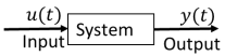
Here we have a very simple process model: an input $ u(t) $ is manipulated by a $ System $ to produce an output $ y(t) $.
A set of differential equations are commonly used to model the system, which then gives the response in time domain. However this method gives very limited information on the predictable system behaviours.
2. Block Diagram
- Rationale: Compartmentalise different components of the system
- Processes = System/Plant $ G(s) $
- Input-output = measurable variables eg. molecules production, genes transcription/translation events or any physical quantities
- In a closed-loop system, a sensor for the output signal sends back information to determine the error between the actual and desired output.
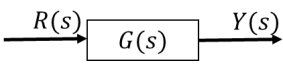
Open Loop System
In the open loop system presented here, $ R(s) $ is the input to the plant $ G(s) $ to give the output $ Y(s) $. This gives the relationship of $ Y(s) = G(s) R(s) $. Hence, the plant is $ G(s)=\frac{Y(s)}{R(s)}$
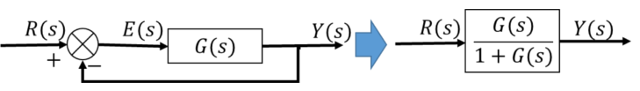
Closed Loop System
In the closed loop system: $ R(s) $ is the reference (desirable) output; $ E(s) $ is the error between the actual and desirable outputs, which in this case acts as the input to the system $ G(s) $.
System analysis rules the following:
$ E(s)=R(s)-Y(s) $
$ Y(s)=G(s)E(s)=G(s)(R(s)-Y(s)) \to Y(s)=\frac{G(s)}{1+G(s)}R(s) $
By this the error term is eliminated to establish the process based on the information of the actual and desirable outputs.
Alternatively, system reduction according to Mason’s rule (as shown on the right of the diagram) gives the following equation for the plant:
$ \frac{Y(s)}{R(s)}=\frac{G(s)}{1+G(s)}$
The Laplace transform of the plant $ G(s) $ can be implemented in MATLAB with the following codes:
Assume $ g(t)=te^{-t} $,
- Root-finding:
- First order polynomial: $ p(s)=As+B $ then $ s=-B/A $
- Second order polynomial: $p(s)=as^{2}+bs+c $ then $ s=\frac{-b\pm\sqrt{b^{2}-4ac}}{2a} $
- Third order polynomial with imaginary roots: $ p(s)=s^{3}+3s^{2}+3s+1+K $ where $ K=j\omega, -j\omega $ then $ p(s)=(s^{2}+\omega^{2})(s+a) $
- Inspect convergence from Pole-Zero Map:
- Usage: Inspect stability and convergence
- Pole = root(s) of the denominator polynomial (‘x’)
- Zero = root(s) of the numerator polynomial (‘o’)
- MATLAB command
pzmap(sys) - Example:
- $ J(s)=\frac{2(s^{2}-2s+5)}{s(s^{2}+4)} $ has poles (‘x’) at $ 0 $ and $ \pm2j $ and zeros (‘o’) at $ 1\pm2j $
-
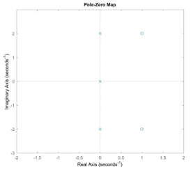
Pole-Zero Map of the system $ J(s)=\frac{2(s^{2}-2s+5)}{s(s^{2}+4)} $
- Properties:
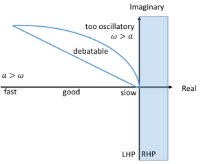
- Right-half plane (RHP) refers to the real part of the root > 0;
- Left-half plane (LHP) refers to the real part of the root < 0.
- We only consider the denominator polynomial (poles) for convergence evaluation:
-
1st Order Polynomial 2nd Order Polynomial Attribute s+a All additive terms Root in LHP $ \to $ Convergent s-b Contain subtractive terms Root in RHP $ \to $ Divergent - For third order polynomial: according the Routh array, for $ P(s) = As^{3}+Bs^{2}+Cs+D $, $ P(s) $ has all roots in LHP only if $ AD < BC $
-
Pole position gives an insight on the system behaviour. This diagram roughly defines the regions of pole positions with predicted response. RHP is not considered since the systems do not converge (unlike genetic circuits, in engineering, we strive to model stabilisation and convergence!)
Pole-zero map Analysis
- Now we focus on the oscillatory responses by inspecting the characteristics of second order systems:
- We first transform the system into monic form: $ G(s)=\frac{\omega^{2}_{n}}{s^{2}+2\zeta\omega_{n}s+\omega^{2}_n} $
- Damping $ \zeta $: ratio of exponential decay constant to natural frequency: $ \zeta=\frac{|\sigma|}{\omega_n} $ (hence gives system poles at $ -\sigma \pm j \omega $)
- Undamped natural frequency: $ \omega_{n}=\frac{\omega_{d}}{\sqrt{1-\zeta^{2}}} $
- Here are four types systems responses:
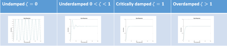
Four Second-Order System Response Types
- Some other specific characteristics which are interesting to look at in Underdamped system ($ 0<\zeta
- Damped natural frequency: $ \omega_{d}=\omega{n}\sqrt{(1-\zeta^2)} $
- Rise time $ T_{r} $: time for the response to go from 10% to the first 90% point of the final value
- Peak time $ T_{p} $: time to the first peak
- Percentage overshoot $ %OS $: highest peak to steady-state value in percentage
- Settling time $ T_{s} $: time for oscillations to reach and stay within 2% (sometimes 5%) of steady-state value
- Ultimately, with all the system analysis tools, we would like to manipulate different blocks of the system to attaindesirable outputs. Given the existing plant, how can we manipulate the system behaviour? What if there are disturbances in the system – how do we reject these disturbances?
- A typical engineering scenario is that, when an aircraft during automatic cruising faces changes in air currents around it, how do different components (engine speed, direction etc.) coordinate to respond and provide a stable flight experience?
4. Controller design
- Controllers are inserted into the system to enhance the plant performance and/or reject disturbances. Here is an overview of the two traditional controller design strategies:
- PID control:
-
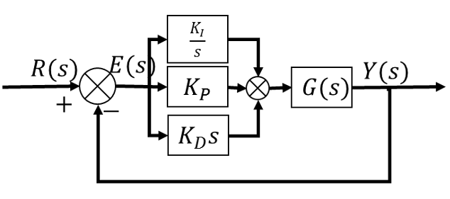
PID Controller acting on a system
-
Control Action Effects on System Response Proportional $ K_{P} $ -Scaling error signal $ \to $ direct effect on steady-state error -Transient response (change $ \zeta $) -Increases oscillations Integral $\frac{K_{I}}{s} $ -Removes steady-state error (operates even when error is 0) -Introduces oscillations -Introduces critically stable pole Derivative $ K_{D}s $ -Damp down oscillations -Provides prediction of future error
-
- Classical control:
- Stability criteria in the frequency domain step up to another level of complexity. In circuits, these controller designs are determined by Root-locus diagram, bode plot (gain and phase margins) and Nyquist criterion. With these indicators, lead compensator $K_{lead}=K\frac{s+a}{s+ra} $ and lag compensator $K_{lag}=K\frac{s+ra}{s+a} $ are chosen to bring about desirable system response in terms of the bandwidth, high- and low- frequency gains (final steady states) and so on.
- Controller design in MATLAB is simple with the toolbox:
simulink - Outlook: Designing compensators to drive desirable system response can give us an insight into how other components in the biological system (which had not been considered in the main system plant $G(s) $) are contributing to the system. For instance, the need to introduce a lead compensator (which speeds up response) might translate to the fact that some biological factors unknown to the system (ie. not represented in the system) are acting to speed up the responses from known compensators.