Interpolation function
- Defines the type of polynomials used approximate the real solution
- Higher order polynomials have some flexibilities to approximate the actual solution more accurately
- However it requires more information and operations to compute a higher order element. For example, in 1D, a 2nd order function requires information from 3 nodes to determine the 3 constants:
- $ \phi = \alpha_1 + \alpha_2 x $ for 2 nodes
- $ \phi = \alpha_1 + \alpha_2 x + \alpha_3 x^2$ for 3 nodes

Upper: 2-node element; Lower: 3-node element
- In 2D, a simple linear equation would have requried 3 nodes to inform the 3 parameters:
- $\phi = \alpha_1 + \alpha_2 x + \alpha_3 y$ for 3 nodes
- $ \phi = \alpha_1 + \alpha_2 x + \alpha_3 y + \alpha_4 xy + \alpha_5 x^2 + \alpha_6 y^2$ for 6 nodes

Upper: 3-node 2D element for linear interpolation function; Lower: 6-node 2D element for quadratic interpolation function
Example problem: Plane Stress/Strain and Isotropic Elasticity
We try to minimise the potential energy $ \Pi $ of the system:
$ \Pi = \Lambda – W $
where $ \Lambda$ is the strain energy of the structure and $ W$ is the work done by external force.
Strain Energy
To calculate the strain energy of the structure $ \Lambda$, we have $ \Lambda = \int_{V} \frac{1}{2} \varepsilon^T \sigma dV$.
- For 1D linear elasticity, we have $ \sigma = E\varepsilon$.
- For 2D linear elasticity, we have $ \mathbf{\sigma} = \mathbf{D\varepsilon}$.
- Inside this equation:
- $ \mathbf{\sigma}^T = \begin{Bmatrix} \sigma_x & \sigma_y & \tau_{xy} \end{Bmatrix}$
- For Plane stress: $ \mathbf{D} = \frac{E}{(1-v^2)} \begin{bmatrix} 1 & v & 0 \\ v & 1 & 0 \\ 0 & 0 & \frac{1-v}{2} \end{bmatrix} $
- For Plane strain: $ \mathbf{D} = \frac{E}{(1+v)(1-2v)} \begin{bmatrix} 1-v & v & 0 \\ v & 1-v & 0 \\ 0 & 0 & \frac{1-2v}{2} \end{bmatrix} $
- $ \mathbf{\varepsilon}^T = \begin{Bmatrix} \varepsilon_x & \varepsilon_y & \gamma_{xy}\end{Bmatrix}$
At each node: $ \mathbf{u = Nu_e}$
- $ \mathbf{u_e} = \begin{Bmatrix} u_i & v_i & u_j & v_j & … & v_n \end{Bmatrix}$
- Remember the following:
- $\varepsilon_x = \frac{\partial u}{\partial x}$
- $\varepsilon_y = \frac{\partial v}{\partial y}$
- $\gamma_{xy} = \frac{\partial u}{\partial y} + \frac{\partial v}{\partial x}$
- After differentiation, $\mathbf{\varepsilon = Bu_e}$
- ie. for a 2-D triangular element: $u = N_iu_i+N_ju_j+N_ku_k$
- $\varepsilon_x = \frac{\partial u}{\partial x} = \frac{\partial N_i}{\partial x}u_i+\frac{\partial N_j}{\partial x}u_j+\frac{\partial N_k}{\partial x}u_k$
For simplex elements, $ \frac{\partial \mathbf{N}}{\partial x}$ return constants.
Then it sums up to the element stiffness matrix $ \mathbf{K_e}$:
$ \Lambda = \frac{1}{2} \int_{V_e} \mathbf{u^T_e} \mathbf{B^T} \mathbf{DBu_e} dV_e = \frac{1}{2}\mathbf{u}^T_e \mathbf{u}_e \mathbf{K_e}$
where $ \mathbf{K_e} = \int_{V_e} \mathbf{B^T DB} dV_e$.
Work done by external force
For simplicity, we assume a nodal load: $ W = \mathbf{u^T_ef_e}$
Assembling the equations of the entire system:
$ \Pi = \sum^{E}_{e=1} \frac{1}{2} \mathbf{u^T_eK_eu_e} – \mathbf{u^T_ef_e}$
To get:
$ \frac{\partial \Pi}{\partial U} = \sum^{E}_{e=1} \mathbf{K_eU}-\mathbf{F} = 0$
$ \mathbf{K} = \sum^{E}_{e=1} \mathbf{K_e}$ is called the global stiffness matrix.
2D Simplex elements
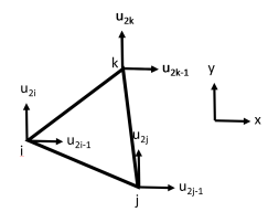
2D Simplex element definition
Nodal information: $ \begin{Bmatrix}u \\ v \end{Bmatrix} = \begin{bmatrix} N_i & 0 & N_j & 0 & N_k & 0 \\ 0 & N_i & 0 & N_j & 0 & N_k \end{bmatrix} \begin{Bmatrix} u_{2i-1} \\ u_{2i} \\u_{2j-1} \\ u_{2j} \\u_{2k-1} \\ u_{2k} \end{Bmatrix} = \mathbf{Nu_e}$
Shape function: $ N_\beta = \frac{1}{2A}(a_\beta+b_\beta x+c_\beta y) for \beta \in \{i,j,k\}$
Nodal Strain:
- $\varepsilon_x = \begin{bmatrix} \frac{\partial N_i}{\partial x} & 0 & \frac{\partial N_j}{\partial x} & 0 & \frac{\partial N_k}{\partial x} & 0 \end{bmatrix} \mathbf{u_e} = \frac{1}{2A} \begin{bmatrix} b_i & 0 & b_j & 0 & b_k & 0 \end{bmatrix} \mathbf{u_e}$
- $\varepsilon_y = \begin{bmatrix} 0 & \frac{\partial N_i}{\partial y} & 0 & \frac{\partial N_j}{\partial y} & 0 & \frac{\partial N_k}{\partial y} \end{bmatrix} \mathbf{u_e} = \frac{1}{2A} \begin{bmatrix} 0 & c_i & 0 & c_j & 0 & c_k \end{bmatrix} \mathbf{u_e}$
- $\gamma_{xy} = \begin{bmatrix} \frac{\partial N_i}{\partial y} & \frac{\partial N_i}{\partial x} & \frac{\partial N_j}{\partial y} & \frac{\partial N_i}{\partial x} & \frac{\partial N_k}{\partial y} & \frac{\partial N_i}{\partial x} \end{bmatrix} \mathbf{u_e} = \frac{1}{2A} \begin{bmatrix} c_i & b_i & c_j & b_j & c_k & b_k \end{bmatrix} \mathbf{u_e}$
- Boom!
- Assemble these equations to give $\mathbf{B}$:
- $\begin{Bmatrix} \varepsilon_x \\ \varepsilon_y \\ \gamma_{xy} \end{Bmatrix} = \frac{1}{2A} \begin{bmatrix} b_i & 0 & b_j & 0 & b_k & 0 \\ 0 & c_i & 0 & c_j & 0 & c_k \\ c_i & b_i & c_j & b_j & c_k & b_k \end{bmatrix} \mathbf{u_e} = \mathbf{Bu_e}$
Get $ \mathbf{K} $:
$ \mathbf{K_e} = \int_V \mathbf{B^T DB} dV = \mathbf{B^T DB} \int_V dV = \mathbf{B^T DB} tA $
where $ t$ is the thickness, and $ A$ is the element area.
Now we get $ \mathbf{K_e}$, how do we construct $latex \mathbf{K} = \sum^{E}_{e=1} \mathbf{K_e}$?
We do a numerical integration using Gaussian quadrature:
$ \int^1_{-1} f(x) dx = \sum^n_{i=1} w_i f(x_i)$
which means that we numerically integrate function $ f(x)$ by summing up the function output $ f(x_i)$ at sample points $ x_i$ multiplied by the corresponding weights $ w_i$. $ n$ is the number of sample points.
The weight $ w_i$ is calculated by $ w_i = \frac{2}{(1-x_i^2)(P’_n (x_i))^2}$ with $ P_n(x)$ being the Legendre polynomial. Or (a look-up table):
| No. of points $ n$ | Points $ x_i$ | Weights $ w_i$ |
|---|---|---|
| 1 | 0 | 2 |
| 2 | $ \pm \sqrt{\frac{1}{3}}$ | 1 |
| 3 | 0 | $ \frac{8}{9}$ |
| $ \pm \sqrt{\frac{3}{5}} $ | $ \frac{5}{9}$ | |
| 4 | $ \pm \sqrt{\frac{3}{7}-\frac{2}{7}\sqrt{\frac{6}{5}}}$ | $ \frac{18+\sqrt{30}}{36}$ |
| $ \pm \sqrt{\frac{3}{7}-\frac{2}{7}\sqrt{\frac{6}{5}}}$ | $ \frac{18-\sqrt{30}}{36}$ | |
| 5 | 0 | $ \frac{128}{225}$ |
| $ \pm \frac{1}{3} \sqrt{5-2\sqrt{\frac{10}{7}}}$ | $ \frac{322+13\sqrt{70}}{900}$ | |
| $ \pm \frac{1}{3} \sqrt{5+2\sqrt{\frac{10}{7}}}$ | $ \frac{322-13\sqrt{70}}{900}$ |
This sets up the global stiffness matrix. Together with boundary conditions, initial conditions and the finite element mesh, we can solve the linear/non-linear matrix to obtain nodal results. This current example is a linear model. We will soon explore a non-linear mechanical model.
Sources:
- Endre Suli’s Lecture notes on Finite Element Methods for Partial Differential Equations
- Endre Suli and David Mayers – An Introduction to Numerical Analysis